The spirit of these notes is to be brief, to give examples and to pull together useful formulas. The references given in the Analysis Page give more detailed discussions. We also include here the sections on probability and statistics from the Particle Data Group at Lawrence Berkeley Lab. These notes are fairly comprehensive and succint.
It takes a while to gain an appreciation of the whole measurement process which involves not only getting a number for the final answer - but also a quote on how precise that number is. In physics this is critical, especially when making a measurement to test or challenge a theory. It is not sufficient to quote how close or far your measurement is from the theoretical expectation - but also how significant the distance from the true answer is. That depends on the precision with which the quantity is measured.
Precision and accuracy have special meaning when discussing measurements and errors. The precision of a measurement of a quantity tells how well the quantity has been measured without any reference to the true value of the quantity. The accuracy tells how close the measurement is to the true value. So you can be precise and very inaccurate - i.e., precisely wrong. For example, suppose you are doing an optics experiment with a light source, lens and screen. You could measure the distance between the light source and screen to fraction of a millimeter accuracy using a machinist's rule but forget to take into account that the actually light source is several centimeters inside the box which contains it. Your measurement of the distance would be very precise (better than a fraction of a millimeter) and also very inaccurate (worse than a centimeter).
Precision is set by random measurement errors and accuracy by systematic errors.
Random errors are due to inherent limitations in measuring devices. Suppose you are measuring the length of an object with a ruler which has marks every 0.5 inch. The precision of the meaurement of the length of the object is set by the fact that you need to estimate the position of one end of the object between adjacent marks on the ruler separated by 0.5 inch. One technique to improve the measurement is to ask several people to make measurements and then take the average. Another is to get a ruler with finer markings. So random errors are determined by technique and the inherent precision of the measuring instrument.
Another example is measuring time between two events, say light on and light off. Suppose you were using an analog watch with no second hand. The precision of your measurement of the interval would be dominated by the ability to estimate the movement of the minute hand - assuming there were minute tic marks on the watch face. It you were now given a digital stop watch with a display showing seconds and 10's of milliseconds as well you would be more precise - and now your precision would likely be limited by your reaction time to the light turning on and then turning off.
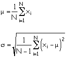
If measurements of a quantity are truly random, the distribution of measurements are distributed about the mean (average) of the measurements. The distribution of the measurements, when plotted as a histogram, follows a Gaussian or normal distribution. Suppose we make N measurements of a the variable, x. The mean of the measurements is denoted by the Greek letter "mu" and the spread of measurements is characterized bu the Greek letter "sigma." Here is how "mu" and "sigma" are calculated:

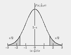
The "sigma" characterizes the spread of measurements. Here is what this means, quantitatively. The Gaussian distribution is given by:
Using this you can estimate the probability that a measurement of x will yield a value a given distance from the mean. That is, suppose that you quote a measurement and its error as:
Suppose we wanted the probability that another random measurement of x would yield a value which is 2*sigma away from the quoted mean. You would find the area under the Gaussian from:

From the table below you see that corresponds to 4.5 % of the total area or, in other words, there is a 95 % probability that a measurement of x will be within 2*sigma away from the mean.


By the way, the error in the mean is given by:
so it pays to average - and to make many measurements. By making more measurements you improve the statistical precision.
Systematic measurement errors are reproducible and are due to faulty equipment, calibration or technique. For example, in our discussion of random errors we gave examples involving use of a ruler and a clock. The scale on the ruler could be incorrectly calibrated because it is made of wood and the wood shrunk from the time it was originally made. The watch could be faulty because of a bad internal clock spring. These would lead to measurements whose precision would not change but whose accuracy would be degraded.
Very often a measurement of a quantity depends on a direct measurement of two other quantities. For example, Snell's law relates the incident angle (i) and refracted angle (r) and the index of refraction (n):
The quantity of interest is n and we would also like to know the error in n. However, n is not measured directly - rather the angles, i and r are measured, each with a certain measurement error. How does one estimate the error in n?
We will formulate the question this way: suppose a quantity f depends on a measurement of x and y. The quantities x and y are measured directly and the measurement errors are determined. What is the error in f? A summary of useful formulas is given here.